本节需要的函数
基本函数(阶跃、gimomid等)
1
2
3
4
5
6
7
8
9
10
11
12
13
14
15
16
17
18
19
20
21
22
23
24
25
26
27
28
29
30
31
32
33
34
35
36
37
38
39
40
41
42
43
44
45
46
47
48
49
50
51
52
53
54
55
56
57
58
59
60
61
62
63
64
65
66
67
68
69
70
71
72
73
74
75
76
77
78
79
80
import numpy as np


def identity_function(x):
    return x


def step_function(x):
    return np.array(x > 0, dtype=np.int)


def sigmoid(x):
    return 1 / (1 + np.exp(-x))


def sigmoid_grad(x):
    return (1.0 - sigmoid(x)) * sigmoid(x)


def relu(x):
    return np.maximum(0, x)


def relu_grad(x):
    grad = np.zeros(x)
    grad[x>=0] = 1
    return grad


def softmax(x):
    if x.ndim == 2:
        x = x.T
        x = x - np.max(x, axis=0)
        y = np.exp(x) / np.sum(np.exp(x), axis=0)
        return y.T

    x = x - np.max(x) # 溢出对策
    return np.exp(x) / np.sum(np.exp(x))


def mean_squared_error(y, t):
    return 0.5 * np.sum((y-t)**2)


def cross_entropy_error(y, t):
    if y.ndim == 1:
        t = t.reshape(1, t.size)
        y = y.reshape(1, y.size)

    # 监督数据是one-hot-vector的情况下,转换为正确解标签的索引
    if t.size == y.size:
        t = t.argmax(axis=1)

    batch_size = y.shape[0]
    return -np.sum(np.log(y[np.arange(batch_size), t] + 1e-7)) / batch_size


def softmax_loss(X, t):
    y = softmax(X)
    return cross_entropy_error(y, t)

def numerical_gradient(f, x):
    h = 1e-4 # 0.0001
    grad = np.zeros_like(x)

    it = np.nditer(x, flags=['multi_index'], op_flags=['readwrite'])
    while not it.finished:
        idx = it.multi_index
        tmp_val = x[idx]
        x[idx] = float(tmp_val) + h
        fxh1 = f(x) # f(x+h)

        x[idx] = tmp_val - h
        fxh2 = f(x) # f(x-h)
        grad[idx] = (fxh1 - fxh2) / (2*h)

        x[idx] = tmp_val # 还原值
        it.iternext()

    return grad
数值微分求梯度
1
2
3
4
5
6
7
8
9
10
11
12
13
14
15
16
17
18
19
20
21
22
23
24
25
26
27
28
29
30
31
32
33
34
35
36
37
38
39
40
41
42
43
44
45
46
47
48
49
def _numerical_gradient_1d(f, x):
    h = 1e-4 # 0.0001
    grad = np.zeros_like(x)

    for idx in range(x.size):
        tmp_val = x[idx]
        x[idx] = float(tmp_val) + h
        fxh1 = f(x) # f(x+h)

        x[idx] = tmp_val - h
        fxh2 = f(x) # f(x-h)
        grad[idx] = (fxh1 - fxh2) / (2*h)

        x[idx] = tmp_val # 还原值

    return grad


def numerical_gradient_2d(f, X):
    if X.ndim == 1:
        return _numerical_gradient_1d(f, X)
    else:
        grad = np.zeros_like(X)

        for idx, x in enumerate(X):
            grad[idx] = _numerical_gradient_1d(f, x)

        return grad


def numerical_gradient(f, x):
    h = 1e-4 # 0.0001
    grad = np.zeros_like(x)

    it = np.nditer(x, flags=['multi_index'], op_flags=['readwrite'])
    while not it.finished:
        idx = it.multi_index
        tmp_val = x[idx]
        x[idx] = float(tmp_val) + h
        fxh1 = f(x) # f(x+h)

        x[idx] = tmp_val - h
        fxh2 = f(x) # f(x-h)
        grad[idx] = (fxh1 - fxh2) / (2*h)

        x[idx] = tmp_val # 还原值
        it.iternext()

    return grad
加载MNIST数据集
1
2
3
4
5
6
7
8
9
10
11
12
13
14
15
16
17
18
19
20
21
22
23
24
25
26
27
28
29
30
31
32
33
34
35
36
37
38
39
40
41
42
43
44
45
46
47
48
49
50
51
52
53
54
55
56
57
58
59
60
61
62
63
64
65
66
67
68
69
70
71
72
73
74
75
76
77
78
79
80
81
82
83
84
85
86
87
88
89
90
91
92
93
94
95
96
97
98
99
100
101
102
103
104
105
106
107
108
109
110
111
112
113
114
115
116
117
118
119
120
121
122
123
124
125
126
127
128
129
130
131
132
133
try:
    import urllib.request
except ImportError:
    raise ImportError('You should use Python 3.x')
import os.path
from IPython.terminal.embed import InteractiveShellEmbed
import gzip
import pickle
import os
import numpy as np


url_base = 'http://yann.lecun.com/exdb/mnist/'
key_file = {
    'train_img':'train-images-idx3-ubyte.gz',
    'train_label':'train-labels-idx1-ubyte.gz',
    'test_img':'t10k-images-idx3-ubyte.gz',
    'test_label':'t10k-labels-idx1-ubyte.gz'
}

## if you run in terminal, run this
# dataset_dir = os.path.dirname(os.path.abspath(__file__))
## if you run in IPython, run this
ip_shell = InteractiveShellEmbed()
dataset_dir = ip_shell.magic("%pwd")

save_file = dataset_dir + "/mnist.pkl"

train_num = 60000
test_num = 10000
img_dim = (1, 28, 28)
img_size = 784


def _download(file_name):
    file_path = dataset_dir + "/" + file_name

    if os.path.exists(file_path):
        return

    print("Downloading " + file_name + " ... ")
    urllib.request.urlretrieve(url_base + file_name, file_path)
    print("Done")

def download_mnist():
    for v in key_file.values():
       _download(v)

def _load_label(file_name):
    file_path = dataset_dir + "/" + file_name

    print("Converting " + file_name + " to NumPy Array ...")
    with gzip.open(file_path, 'rb') as f:
            labels = np.frombuffer(f.read(), np.uint8, offset=8)
    print("Done")

    return labels

def _load_img(file_name):
    file_path = dataset_dir + "/" + file_name

    print("Converting " + file_name + " to NumPy Array ...")
    with gzip.open(file_path, 'rb') as f:
            data = np.frombuffer(f.read(), np.uint8, offset=16)
    data = data.reshape(-1, img_size)
    print("Done")

    return data

def _convert_numpy():
    dataset = {}
    dataset['train_img'] =  _load_img(key_file['train_img'])
    dataset['train_label'] = _load_label(key_file['train_label'])
    dataset['test_img'] = _load_img(key_file['test_img'])
    dataset['test_label'] = _load_label(key_file['test_label'])

    return dataset

def init_mnist():
    download_mnist()
    dataset = _convert_numpy()
    print("Creating pickle file ...")
    with open(save_file, 'wb') as f:
        pickle.dump(dataset, f, -1)
    print("Done!")

def _change_one_hot_label(X):
    T = np.zeros((X.size, 10))
    for idx, row in enumerate(T):
        row[X[idx]] = 1

    return T


def load_mnist(normalize=True, flatten=True, one_hot_label=False):
    """读入MNIST数据集

    Parameters
    ----------
    normalize : 将图像的像素值正规化为0.0~1.0
    one_hot_label :
        one_hot_label为True的情况下,标签作为one-hot数组返回
        one-hot数组是指[0,0,1,0,0,0,0,0,0,0]这样的数组
    flatten : 是否将图像展开为一维数组

    Returns
    -------
    (训练图像, 训练标签), (测试图像, 测试标签)
    """
    if not os.path.exists(save_file):
        init_mnist()

    with open(save_file, 'rb') as f:
        dataset = pickle.load(f)

    if normalize:
        for key in ('train_img', 'test_img'):
            dataset[key] = dataset[key].astype(np.float32)
            dataset[key] /= 255.0

    if one_hot_label:
        dataset['train_label'] = _change_one_hot_label(dataset['train_label'])
        dataset['test_label'] = _change_one_hot_label(dataset['test_label'])

    if not flatten:
         for key in ('train_img', 'test_img'):
            dataset[key] = dataset[key].reshape(-1, 1, 28, 28)

    return (dataset['train_img'], dataset['train_label']), (dataset['test_img'], dataset['test_label'])


if __name__ == '__main__':
    init_mnist()
计算图
尽管我们学过求导和链式求导法则,但我们依然要说说这个。因为很多深度学习框架就是靠这个来进行随机梯度下降(SGD)的。
什么是计算图?假如我们有一个算式:$p=x+y$,我们可以用类似于神经元的方式画出这样的图:

图中,每个节点是一个算符,算符对输入的数据进行计算,再输出值。通过多个算符的组合,可以表示出复杂的式子,比如:$(x+y)\times z$

计算图既可以将简单的计算组合起来,也可以将复杂的计算分解为简单的计算。
从计算图的出发点到结束点的传播称为正向传播(forward propagation),从结束点向出发点传播,则为反向传播(backward propagation)。正向传播很好计算,但反向传播又如何计算呢?我们之前学过的求导的链式法则就派上用场了。
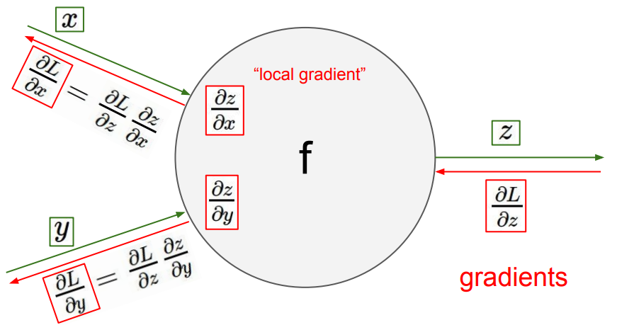
假如我们有一个节点是:$z=f(x,y)$,现在我们反向传播,已知了 $\dfrac{\partial L}{\partial z}$,现在要求 $\dfrac{\partial L}{\partial x}$,可以通过 $\dfrac{\partial L}{\partial z}\cdot\dfrac{\partial z}{\partial x}$ 得到。以上面那个 $(x+y)\times z$ 为例:
- 先考虑 g 到 p 的反向传播:$\dfrac{\partial g}{\partial p}=z$
- 然后再考虑 p 到 x 的反向传播:$\dfrac{\partial p}{\partial x}=1$
- 将两个组合起来:$\dfrac{\partial g}{\partial p} \cdot \dfrac{\partial p}{\partial x}= z$
可见,反向传播同正向传播一样,也是可以将简单的求导组合起来,得到输出到输入的求导。我们可以将中间变量储存起来,进行多次利用,从而节省求导时间。
简单层的实现
乘法层和加法层
乘法层:
\[z=x\cdot y\\ \frac{\partial z}{\partial x}=y\\ \frac{\partial z}{\partial y}=x\]加法层:
\[z=x+ y\\ \frac{\partial z}{\partial x}=1\\ \frac{\partial z}{\partial y}=1\]class MulLayer:
def __init__(self):
self.x = None
self.y = None
def forward(self, x, y):
self.x = x
self.y = y
out = x * y
return out
def backward(self, dout):
dx = dout * self.y
dy = dout * self.x
return dx, dy
class AddLayer:
def __init__(self):
pass
def forward(self, x, y):
out = x + y
return out
def backward(self, dout):
dx = dout * 1
dy = dout * 1
return dx, dy
ReLU层
\[y= \begin{cases} x, & (x>0)\\ 0, & (x\leq 0) \end{cases}\\ \frac{\partial y}{\partial x}=\begin{cases} 1, & (x>0)\\ 0, & (x\leq 0) \end{cases}\]import numpy as np
class Relu:
def __init__(self):
self.mask = None
def forward(self, x):
self.mask = (x <= 0)
out = x.copy()
out[self.mask] = 0 #将小于0的x对应的输出置0
return out
def backward(self, dout):
dout[self.mask] = 0
dx = dout
return dx
Sigmoid层
\[y=\frac{1}{1+\exp(-x)}\\ \frac{\partial y}{\partial x}=\frac{\exp(-x)}{[1+\exp(-x)]^2}=y(1-y)\]class Sigmoid:
def __init__(self):
self.out = None
def forward(self, x):
out = sigmoid(x)
self.out = out
return out
def backward(self, dout):
dx = dout * (1.0 - self.out) * self.out
return dx
Affine层
Affine 层包含多个权重以及偏置,其求导也相对复杂得多
\[\newcommand{\bd}{\boldsymbol}\] \[\bd{X}\cdot\bd{W}+\bd{B}=\bd{Y}\]我们不妨假设:
\[\begin{bmatrix} x_1 & x_2 \end{bmatrix} \cdot \begin{bmatrix} w_{11} & w_{12} & w_{13}\\ w_{21} & w_{22} & w_{23} \end{bmatrix} + \begin{bmatrix} b_1 & b_2 & b_3 \end{bmatrix}= \begin{bmatrix} y_1 & y_2 & y_3 \end{bmatrix}\]根据矩阵的求导法则,如果我们采用分子布局(求导时分子相同的放同一行):
\[\dfrac{\partial \bd{Y}}{\partial \bd{X}} = \begin{bmatrix} \dfrac{\partial y_1}{\partial x_1} & \dfrac{\partial y_1}{\partial x_2} \\ \dfrac{\partial y_2}{\partial x_1} & \dfrac{\partial y_2}{\partial x_2} \\ \dfrac{\partial y_3}{\partial x_1} & \dfrac{\partial y_3}{\partial x_2} \end{bmatrix} = \begin{bmatrix} w_{11} & w_{21} \\ w_{12} & w_{22} \\ w_{13} & w_{23} \end{bmatrix} = \bd{W}^T\]同理:
\[\dfrac{\partial \bd{Y}}{\partial \bd{W}} = \bd{X}^T \quad \dfrac{\partial \bd{Y}}{\partial \bd{B}} = \bd{1}\]但要注意,如果考虑 $\bd{Y}$ 反向传播之前的求导,即求:$\dfrac{\partial L}{\partial \bd{X}}$ 和 $\dfrac{\partial L}{\partial \bd{W}}$,则还要考虑矩阵乘法的顺序:
\[\dfrac{\partial L}{\partial \bd{X}} = \dfrac{\partial L}{\partial \bd{Y}} \cdot \bd{W}^T\\ \dfrac{\partial L}{\partial \bd{W}} = \bd{X}^T \cdot \dfrac{\partial L}{\partial \bd{Y}}\]从行列数匹配的角度去想会好理解一点。因为 $\dfrac{\partial L}{\partial \bd{X}} = \begin{bmatrix}\dfrac{\partial L}{\partial x_1} & \dfrac{\partial L}{\partial x_2} \end{bmatrix}$,$\dfrac{\partial L}{\partial \bd{W}} = \begin{bmatrix}\dfrac{\partial L}{\partial w_1} & \dfrac{\partial L}{\partial w_2} & \dfrac{\partial L}{\partial w_3}\end{bmatrix}$,而 $\dfrac{\partial \bd{Y}}{\partial \bd{X}}= \bd{W}^T$ 是一个 $3\times2$ 的矩阵,所以必须是 $\dfrac{\partial L}{\partial \bd{X}} = \dfrac{\partial L}{\partial \bd{Y}} \cdot \bd{W}^T$。另一个也是一样的道理,但写起来稍微复杂一点,在这里就不写了。
如果考虑 $\bd{X}$ 是二维、三维、四维的情况,那么我们对偏置求偏导时,需要将 $\dfrac{\partial L}{\partial \bd{Y}}$ 0维对应的数据相加,即:$\dfrac{\partial L}{\partial \bd{B}} = \begin{bmatrix}\sum\dfrac{\partial L}{\partial y_{i1}} & \sum \dfrac{\partial L}{\partial x_{i2}} & \cdots \end{bmatrix}$。这是因为对于多维的情况,偏置$\bd{B}$ 会先进行扩充,然后再相加到各个数据上,所以反过来,求导的时候则需要合并。
下面是批处理版本的代码。
class Affine:
    def __init__(self, W, b):
        self.W = W #权重
        self.b = b #偏置

        self.x = None #输入
        self.original_x_shape = None #原输入的形状
        # 权重和偏置参数的导数
        self.dW = None
        self.db = None

    def forward(self, x):
        # 对应张量
        self.original_x_shape = x.shape
        x = x.reshape(x.shape[0], -1)
        self.x = x

        out = np.dot(self.x, self.W) + self.b

        return out

    def backward(self, dout):
        dx = np.dot(dout, self.W.T) #对应上面的公式
        self.dW = np.dot(self.x.T, dout) #对应上面的公式
        self.db = np.sum(dout, axis=0)

        dx = dx.reshape(*self.original_x_shape)  # 还原输入数据的形状(对应张量)
        return dx
Softmax 层
\[y_k = \frac{\exp(a_k)}{\sum_{i=1}^n \exp(a_i)}\]一般我们会结合 loss 层一起考虑。
class SoftmaxWithLoss:
    def __init__(self):
        self.loss = None
        self.y = None # softmax的输出
        self.t = None # 监督数据

    def forward(self, x, t):
        self.t = t
        self.y = softmax(x)
        self.loss = cross_entropy_error(self.y, self.t)

        return self.loss

    def backward(self, dout=1):
        batch_size = self.t.shape[0]
        if self.t.size == self.y.size: # 监督数据是one-hot-vector的情况
            dx = (self.y - self.t) / batch_size
        else:
            dx = self.y.copy()
            dx[np.arange(batch_size), self.t] -= 1
            dx = dx / batch_size

        return dx
误差反向传播算法的实现
与之前一样,我们同样是生成一个两层的神经网络,唯一不同的是,神经网络增加了一个误差反向传播求梯度的函数
from collections import OrderedDict

class TwoLayerNet:

    def __init__(self, input_size, hidden_size, output_size, weight_init_std = 0.01):
        # 初始化权重
        self.params = {}
        self.params['W1'] = weight_init_std * np.random.randn(input_size, hidden_size)
        self.params['b1'] = np.zeros(hidden_size)
        self.params['W2'] = weight_init_std * np.random.randn(hidden_size, output_size)
        self.params['b2'] = np.zeros(output_size)

        # 生成层
        self.layers = OrderedDict()
        self.layers['Affine1'] = Affine(self.params['W1'], self.params['b1'])
        self.layers['Relu1'] = Relu()
        self.layers['Affine2'] = Affine(self.params['W2'], self.params['b2'])

        self.lastLayer = SoftmaxWithLoss()

    def predict(self, x):
        for layer in self.layers.values():
            x = layer.forward(x)

        return x

    # x:输入数据, t:监督数据
    def loss(self, x, t):
        y = self.predict(x)
        return self.lastLayer.forward(y, t)

    def accuracy(self, x, t):
        y = self.predict(x)
        y = np.argmax(y, axis=1)
        if t.ndim != 1 : t = np.argmax(t, axis=1)

        accuracy = np.sum(y == t) / float(x.shape[0])
        return accuracy

    # x:输入数据, t:监督数据
    def numerical_gradient(self, x, t):
        loss_W = lambda W: self.loss(x, t)

        grads = {}
        grads['W1'] = numerical_gradient(loss_W, self.params['W1'])
        grads['b1'] = numerical_gradient(loss_W, self.params['b1'])
        grads['W2'] = numerical_gradient(loss_W, self.params['W2'])
        grads['b2'] = numerical_gradient(loss_W, self.params['b2'])

        return grads

    def gradient(self, x, t):
        # forward
        self.loss(x, t)

        # backward
        dout = 1
        dout = self.lastLayer.backward(dout)

        layers = list(self.layers.values())
        layers.reverse()
        for layer in layers:
            dout = layer.backward(dout)

        # 设定
        grads = {}
        grads['W1'], grads['b1'] = self.layers['Affine1'].dW, self.layers['Affine1'].db
        grads['W2'], grads['b2'] = self.layers['Affine2'].dW, self.layers['Affine2'].db

        return grads
训练网络:
(x_train, t_train), (x_test, t_test) = load_mnist(normalize=True, one_hot_label=True)

network = TwoLayerNet(input_size=784, hidden_size=50, output_size=10)

iters_num = 10000
train_size = x_train.shape[0]
batch_size = 100
learning_rate = 0.1

train_loss_list = []
train_acc_list = []
test_acc_list = []

iter_per_epoch = max(train_size / batch_size, 1)

for i in range(iters_num):
    batch_mask = np.random.choice(train_size, batch_size)
    x_batch = x_train[batch_mask]
    t_batch = t_train[batch_mask]

    # 梯度
    #grad = network.numerical_gradient(x_batch, t_batch)
    grad = network.gradient(x_batch, t_batch)

    # 更新
    for key in ('W1', 'b1', 'W2', 'b2'):
        network.params[key] -= learning_rate * grad[key]

    loss = network.loss(x_batch, t_batch)
    train_loss_list.append(loss)

    if i % iter_per_epoch == 0:
        train_acc = network.accuracy(x_train, t_train)
        test_acc = network.accuracy(x_test, t_test)
        train_acc_list.append(train_acc)
        test_acc_list.append(test_acc)
        print(train_acc, test_acc)
OUTPUT:
    0.12738333333333332 0.1288
    0.90455 0.909
    0.92495 0.928
    0.9365 0.9395
    0.9444166666666667 0.946
    0.9498 0.9504
    0.9550333333333333 0.9544
    0.9592666666666667 0.9566
    0.95915 0.9562
    0.9624333333333334 0.9585
    0.9674333333333334 0.9643
    0.9693166666666667 0.9628
    0.9727166666666667 0.9672
    0.9727 0.9658
    0.9735166666666667 0.9673
    0.975 0.968
    0.9780833333333333 0.97
我们可以将反向传播与之前的数值微分得到的值进行比较:
# 读入数据
(x_train, t_train), (x_test, t_test) = load_mnist(normalize=True, one_hot_label=True)

network = TwoLayerNet(input_size=784, hidden_size=50, output_size=10)

x_batch = x_train[:3]
t_batch = t_train[:3]

grad_numerical = network.numerical_gradient(x_batch, t_batch)
grad_backprop = network.gradient(x_batch, t_batch)

for key in grad_numerical.keys():
    diff = np.average( np.abs(grad_backprop[key] - grad_numerical[key]) )
    print(key + ":" + str(diff))
OUTPUT
    W1:4.2968520032354943e-10
    b1:2.6641099171273617e-09
    W2:4.796070617839067e-09
    b2:1.3916415531195492e-07
可以发现,两个结果十分相近,说明我们反向传播算法是正确的。