神经网络
从感知机到神经网络
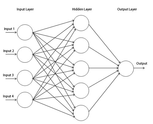
神经网络可以划分为三层:
- 输入层
- 中间层(隐藏层)
- 输出层
一般输入层仅仅是输入数据,并没有对数据进行处理,所以编号为 第0层。总的层数为 3 层,但我们为了于编号一致,将上图中的网络称为 2层网络。
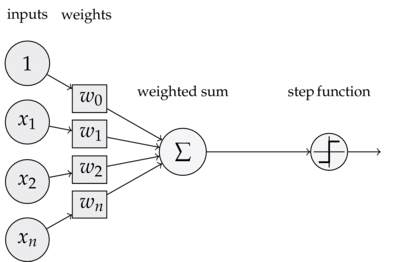
每一层网络由若干个 节点(也叫 神经元)构成,每个节点内部都有相应的处理方法。比如,前面已经学过了感知机的表达式。这里我们对表达式进行拆分:
\[y=h(a)\\ a=b+w_1x_1+w_2x_2\\ h(x)=\begin{cases} 0 & x\leq 0\\ 1 & x > 0 \end{cases}\]我们将 $h(x)$ 称为 激活函数(action function),意思是当输入超出阈值时,就会切换输出值。在感知机中,激活函数是一个阶跃函数。故感知机的节点内部如下图:
常见的激活函数
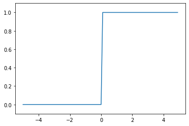
阶跃函数
\[h(x)=\begin{cases} 0 & x\leq 0\\ 1 & x > 0 \end{cases}\]import numpy as np
import matplotlib.pylab as plt
def step_function(x):
return np.array(x > 0, dtype=np.int)
X = np.arange(-5.0, 5.0, 0.1)
Y = step_function(X)
plt.plot(X, Y)
plt.ylim(-0.1, 1.1) # 指定图中绘制的y轴的范围
plt.show()
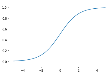
sigmoid 函数
\[h(x)=\frac{1}{1+\exp(-x)}\]import numpy as np
import matplotlib.pylab as plt
def sigmoid(x):
return 1 / (1 + np.exp(-x))
X = np.arange(-5.0, 5.0, 0.1)
Y = sigmoid(X)
plt.plot(X, Y)
plt.ylim(-0.1, 1.1)
plt.show()
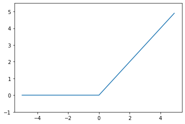
ReLU函数(Rectified Linear Unit)
\[h(x)=\begin{cases} 0 & x\leq 0\\ x & x > 0 \end{cases}\]import numpy as np
import matplotlib.pylab as plt
def relu(x):
return np.maximum(0, x)
x = np.arange(-5.0, 5.0, 0.1)
y = relu(x)
plt.plot(x, y)
plt.ylim(-1.0, 5.5)
plt.show()
我们可以注意到,上面三个都是非线性函数。于是我们就产生了一个问题:能不能用 $y=cx$ 这样的线性函数?显然不能。因为线性函数的叠加依然是线性函数,比如叠加三次 $y=c\times c\times c x=ax$$\;(a=c^3)$,那么我们中间层就完全可以用一层来代替,那么就无法发挥多层网络的优势。
利用矩阵乘法实现神经网络
假如有 2 个输入 $x_1,x_2$ ,3个输出 $y_1,y_2,y_3$,如果要实现:
\[y_1=1x_1+2x_2\\ y_2=3x_1+4x_2\\ y_3=5x_1+6x_3\\\]那么可以写成矩阵相乘:
\[\begin{align} Y&=X \cdot\; W\\ \begin{bmatrix} y_1 & y_2 & y_3 \end{bmatrix}&= \begin{bmatrix} x_1 & x_2 \end{bmatrix}\cdot \begin{bmatrix} 1 & 3 & 5\\ 2 & 4 & 6 \end{bmatrix}\\ 3&=2 \cdot\; 2\times 3 \end{align}\]注意到权重矩阵 $W$ 的行数等于 $X$ 的列数,$W$ 的列数等于 $Y$ 的列数。也就是 $W$ 的形状为 $X_列 \times Y_列$
为了区分不同层,我们在符号的右上角添加数字来表示:$w^{(1)}_{2,3}$ 表示这个权重属于第 1 层,第 2 个神经元,接受的是上一层第 3 个神经元的输入。类似的,$x^{(1)}_1$ 和 $y^{(1)}_1$ 表示第 1 层第 1 个输入或输出。
上面我们忽略了激活函数和偏置,加上激活函数和偏置的表达式应该为:
\[Y=h(A)=h(XW+B)\]比如一个三层的神经网络可以写成:
a1 = np.dot(x, W1) + b1
z1 = sigmoid(a1)

a2 = np.dot(z1, W2) + b2
z2 = sigmoid(a2)

a3 = np.dot(z2, W3) + b3
y = softmax(a3)
输出层
如果是需要具体数字,比如回归预测问题,则激活函数只需要用 恒定函数 即可。
如果是需要概率,比如分类问题,则需要使用 softmax 函数:
\[y_k = \frac{\exp(a_k)}{\sum_{i=1}^n \exp(a_i)}\](使用指数函数是为了使负数 $a_i$ 也可以用于计算概率)
为了避免指数爆炸,一般会减去一个很大的数(结果依然不变):
\[y_k = \frac{\exp(a_k-C)}{\sum_{i=1}^n \exp(a_i-C)}\]import numpy as np
a=np.array([1010,1000,990])
np.exp(a)/np.sum(np.exp(a)) #出现了指数爆炸
OUTPUT:
    /usr/local/lib/python3.6/dist-packages/ipykernel_launcher.py:5: RuntimeWarning: overflow encountered in exp
      """
    /usr/local/lib/python3.6/dist-packages/ipykernel_launcher.py:5: RuntimeWarning: invalid value encountered in true_divide
      """


    array([nan, nan, nan])
c=np.max(a)
np.exp(a-c)/np.sum(np.exp(a-c)) #防止指数爆炸
OUTPUT:
    array([9.99954600e-01, 4.53978686e-05, 2.06106005e-09])
def softmax(x):
    if x.ndim == 2:
        x = x.T
        x = x - np.max(x, axis=0)
        y = np.exp(x) / np.sum(np.exp(x), axis=0)
        return y.T

    x = x - np.max(x) # 溢出对策
    return np.exp(x) / np.sum(np.exp(x))
开始搭建神经网络
手写数字识别
MNIST 手写数字图像集是机器学习最常用的数据集之一。有句话说,如果你的网络在 MNIST 上跑不过,那就别指望它能用。
下面是《深度学习入门》中用于下载和读取 MNIST 的程序。
Load MNIST
1
2
3
4
5
6
7
8
9
10
11
12
13
14
15
16
17
18
19
20
21
22
23
24
25
26
27
28
29
30
31
32
33
34
35
36
37
38
39
40
41
42
43
44
45
46
47
48
49
50
51
52
53
54
55
56
57
58
59
60
61
62
63
64
65
66
67
68
69
70
71
72
73
74
75
76
77
78
79
80
81
82
83
84
85
86
87
88
89
90
91
92
93
94
95
96
97
98
99
100
101
102
103
104
105
106
107
108
109
110
111
112
113
114
115
116
117
118
119
120
121
122
123
124
125
126
127
128
129
130
131
132
133
try:
    import urllib.request
except ImportError:
    raise ImportError('You should use Python 3.x')
import os.path
from IPython.terminal.embed import InteractiveShellEmbed
import gzip
import pickle
import os
import numpy as np


url_base = 'http://yann.lecun.com/exdb/mnist/'
key_file = {
    'train_img':'train-images-idx3-ubyte.gz',
    'train_label':'train-labels-idx1-ubyte.gz',
    'test_img':'t10k-images-idx3-ubyte.gz',
    'test_label':'t10k-labels-idx1-ubyte.gz'
}

## if you run in terminal, run this
# dataset_dir = os.path.dirname(os.path.abspath(__file__))
## if you run in IPython, run this
ip_shell = InteractiveShellEmbed()
dataset_dir = ip_shell.magic("%pwd")

save_file = dataset_dir + "/mnist.pkl"

train_num = 60000
test_num = 10000
img_dim = (1, 28, 28)
img_size = 784


def _download(file_name):
    file_path = dataset_dir + "/" + file_name

    if os.path.exists(file_path):
        return

    print("Downloading " + file_name + " ... ")
    urllib.request.urlretrieve(url_base + file_name, file_path)
    print("Done")

def download_mnist():
    for v in key_file.values():
       _download(v)

def _load_label(file_name):
    file_path = dataset_dir + "/" + file_name

    print("Converting " + file_name + " to NumPy Array ...")
    with gzip.open(file_path, 'rb') as f:
            labels = np.frombuffer(f.read(), np.uint8, offset=8)
    print("Done")

    return labels

def _load_img(file_name):
    file_path = dataset_dir + "/" + file_name

    print("Converting " + file_name + " to NumPy Array ...")
    with gzip.open(file_path, 'rb') as f:
            data = np.frombuffer(f.read(), np.uint8, offset=16)
    data = data.reshape(-1, img_size)
    print("Done")

    return data

def _convert_numpy():
    dataset = {}
    dataset['train_img'] =  _load_img(key_file['train_img'])
    dataset['train_label'] = _load_label(key_file['train_label'])
    dataset['test_img'] = _load_img(key_file['test_img'])
    dataset['test_label'] = _load_label(key_file['test_label'])

    return dataset

def init_mnist():
    download_mnist()
    dataset = _convert_numpy()
    print("Creating pickle file ...")
    with open(save_file, 'wb') as f:
        pickle.dump(dataset, f, -1)
    print("Done!")

def _change_one_hot_label(X):
    T = np.zeros((X.size, 10))
    for idx, row in enumerate(T):
        row[X[idx]] = 1

    return T


def load_mnist(normalize=True, flatten=True, one_hot_label=False):
    """读入MNIST数据集

    Parameters
    ----------
    normalize : 将图像的像素值正规化为0.0~1.0
    one_hot_label :
        one_hot_label为True的情况下,标签作为one-hot数组返回
        one-hot数组是指[0,0,1,0,0,0,0,0,0,0]这样的数组
    flatten : 是否将图像展开为一维数组

    Returns
    -------
    (训练图像, 训练标签), (测试图像, 测试标签)
    """
    if not os.path.exists(save_file):
        init_mnist()

    with open(save_file, 'rb') as f:
        dataset = pickle.load(f)

    if normalize:
        for key in ('train_img', 'test_img'):
            dataset[key] = dataset[key].astype(np.float32)
            dataset[key] /= 255.0

    if one_hot_label:
        dataset['train_label'] = _change_one_hot_label(dataset['train_label'])
        dataset['test_label'] = _change_one_hot_label(dataset['test_label'])

    if not flatten:
         for key in ('train_img', 'test_img'):
            dataset[key] = dataset[key].reshape(-1, 1, 28, 28)

    return (dataset['train_img'], dataset['train_label']), (dataset['test_img'], dataset['test_label'])


if __name__ == '__main__':
    init_mnist()
1
2
3
4
5
6
7
8
9
10
11
12
13
14
15
16
17
18
19
OUTPUT:
    Downloading train-images-idx3-ubyte.gz ...
    Done
    Downloading train-labels-idx1-ubyte.gz ...
    Done
    Downloading t10k-images-idx3-ubyte.gz ...
    Done
    Downloading t10k-labels-idx1-ubyte.gz ...
    Done
    Converting train-images-idx3-ubyte.gz to NumPy Array ...
    Done
    Converting train-labels-idx1-ubyte.gz to NumPy Array ...
    Done
    Converting t10k-images-idx3-ubyte.gz to NumPy Array ...
    Done
    Converting t10k-labels-idx1-ubyte.gz to NumPy Array ...
    Done
    Creating pickle file ...
    Done!
但最好的方式还是通过 tf.keras.datasets.mnist 来使用,这个会自动下载 mnist。
上面的程序中中有用于读取数据的 load_minst() 函数。运行后,它会以“(训练图像,训练标签),(测试图像,测试标签)” 的形式读入。此外,它有三个参数:
normalize=True正规化,即单个像素是 0~255(False) 还是 0~1(True)flatten=True一维化,即是一张 28x28 的图片,还是一张 1x784 的长线one_hot_label=Falseone-hot标签,即标签是 0~9,还是[0,0,1,0,0,0,0,0,0,0]
tf.keras.datasets.mnist 也有 load_minst() 函数,但它不会对数据做任何处理。
下面来读入看一下:
import os
# import tensorflow as tf
import matplotlib.pyplot as plt
# os.environ['TF_CPP_MIN_LOG_LEVEL'] = '2'
# tf.compat.v1.enable_eager_execution()
# print("TensorFlow Version:\t", tf.__version__)
## 加载 MNIST
# mnist = tf.keras.datasets.mnist
## 读入数据
(x_train, y_train), (x_test, y_test) = load_mnist(flatten=False, normalize=True)
print(x_train.shape,
y_train.shape,
x_test.shape,
y_test.shape
) # (60000, 1, 28, 28) (60000,) (10000, 1, 28, 28) (10000,)
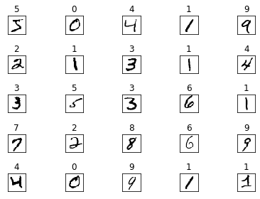
fig, ax = plt.subplots(nrows=5, ncols=5, sharex='all', sharey='all')
ax = ax.flatten()
## 读取前 25 张图
for i in range(25):
img = x_train[i].reshape(28, 28)
ax[i].set_title(y_train[i])
ax[i].imshow(img, cmap='Greys', interpolation='nearest')
ax[0].set_xticks([])
ax[0].set_yticks([])
plt.tight_layout()
plt.show()
OUTPUT:
    (60000, 1, 28, 28) (60000,) (10000, 1, 28, 28) (10000,)
根据数据集,我们可以设计一个含 2 个隐藏层的网络:
- 输入 784
- 隐藏层1 50个神经元 784x50
- 隐藏层2 100个神经元 50x100
- 输出 100x10
def predict(network, x):
    W1, W2, W3 = network['W1'], network['W2'], network['W3']
    b1, b2, b3 = network['b1'], network['b2'], network['b3']

    a1 = np.dot(x, W1) + b1
    z1 = sigmoid(a1)
    a2 = np.dot(z1, W2) + b2
    z2 = sigmoid(a2)
    a3 = np.dot(z2, W3) + b3
    y = softmax(a3)

    return y
由于还没有参数,所以上面的神经网络并不能运行。为了好玩,我们可以选择随机生成参数,比如
(x_train, y_train), (x_test, y_test) = load_mnist(flatten=True, normalize=True, one_hot_label=False)

network={}
network['W1']=np.random.rand(784, 50)
network['W2']=np.random.rand(50, 100)
network['W3']=np.random.rand(100, 10)
network['b1']=np.random.rand(50)
network['b2']=np.random.rand(100)
network['b3']=np.random.rand(10)


accuracy_cnt = 0
for i in range(len(x_test)):
    y = predict(network, x_test[i])
    p= np.argmax(y) # 获取概率最高的元素的索引
    if p == y_test[i]:
        accuracy_cnt += 1

print("Accuracy:" + str(float(accuracy_cnt) / len(x_test)))
OUTPUT:
    Accuracy:0.0958
可见,准确率低得可怜……
上面仅仅是对一个训练样本进行处理。一般训练时,输入时是成“批 patch”输入的,像下面这样:
batch_size = 100 # 批数量
accuracy_cnt = 0


for i in range(0, len(x_test), batch_size):
    x_batch = x_test[i:i+batch_size]
    y_batch = predict(network, x_batch)
    p = np.argmax(y_batch, axis=1)
    accuracy_cnt += np.sum(p == y_test[i:i+batch_size])

print("Accuracy:" + str(float(accuracy_cnt) / len(x_test)))
OUTPUT:
    Accuracy:0.0958